What is Information Entropy?
In this article we would be going over the concept of information entropy, a vital topic in machine learning and information theory.
Table of Contents
What is information theory?
What is expected value (EV)?
Before we understand entropy, a prerequisite is understanding the expected value, a topic in probability theory.
Expected value is a mathematical concept that represents the long-term average or average outcome of a random event or process.
It is calculated by multiplying each possible event outcome by its probability and then summing the results.
It's better to learn this concept with an example.
Let's say you flip an unfair coin, the probability of getting heads is 0.6, and the probability of getting tails is 0.4. If you get tails, you win $10, but if you get heads, you lose $5.
Under these conditions, would you consider playing the game?
We can use the expected value to estimate how much we would be expected to win or lose on average at each round.
Let's say you flip the coin 100 times (100 rounds).
| Heads | Tails | |
| Probability | 0.6 | 0.4 |
| Outcome | - $5 | + $10 |
Based on the above table, in 100 rounds, we would win
\[100 * 0.4 = 40 \text{ rounds} \]
and the amount we would win in 40 rounds, is
\[ 40 * \$10 = \$400 \]
Base on the above table, in 100 rounds, we would lose,
\[100 * 0.6 = 60 \text{ rounds}\]
and the amount we would lose in 60 rounds, is,
\[ 60 * -\$5 = -\$300 \]
If we combine the above deductions into one single expression and divide by 100, we can get the average earnings/losses per round; we get the below expression
\[ \frac{(100 * 0.6 * \$10) + ( 100 * 0.4 * -\$5)}{100} \]
However, we can simplify
\[ \frac{(\cancel{100} * 0.6 * \$10) + ( \cancel{100} * 0.4 * -\$5)}{\cancel{100}} = 0.6 * \$10 + (0.4 * -\$5) = $4\]
Therefore, on average, we earn $4 per round, the expected value (EV) of playing the coin toss game with the unfair coin.
More generally, the expected value can be written as follows,
\[ E[X] = \sum_i x_i * P(X=x_i) \]
X is a random variable (like the coin toss), and \(x_i\) denotes the outcome of the event, which is associated with the random variable (like getting heads or tails at a given moment), and \(P (X=x_i) \) is the probability that you would get heads/tails (e.g., \(P(X = tails) = 0.4 \)
What is entropy?
Entropy is a measure of uncertainty.
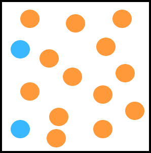
Let's say you have orange and blue balls in a bag, as shown below.
If you randomly select a ball without looking into the bag, there is a higher chance that you will pick an orange color ball.
It is almost certain that you would pick an orange color ball over a blue ball.
Therefore, the uncertainty is low in which ball you would pick.
If you picked an orange ball, you wouldn't be surprised, but if you picked a blue ball you would be surprised.
To break down entropy, we need to understand surprise.
Now let's look at another scenario.
In the below image, there are more blue balls than orange ones.
The probability of picking a blue ball is higher than picking an orange ball.
If we were to pick a blue ball, we wouldn't be that much surprised.
But if we picked an orange ball, we would be very surprised.

So we now think that surprise has an inverse relationship with probability.
A higher probability should make for a lower surprise, and a lower probability should make for a greater surprise.
However, as tempting as this would be, we can't define surprise like this, where \( p(x) \) is the probability of \(x\)
\[ \text{surprise} = \frac{1}{p(x)} \]
The graph for the above function would look something like this,
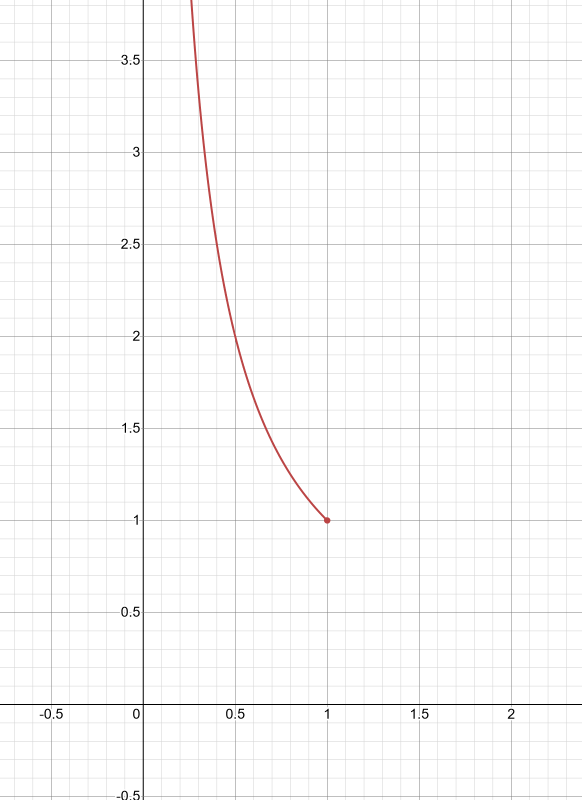
Since probability ranges between 0 and 1, the graph halts at 1.
So if a probability event is certain (i.e., \( p(x) = 1 \)), then the surprise should be zero. Since we won't be surprised, however, the expression we came up with doesn't reflect that.
So, let's take the log of \( \frac{1}{x} \).
\[ \text{surprise} = log (\frac{1}{x}) \]
Here's the graph
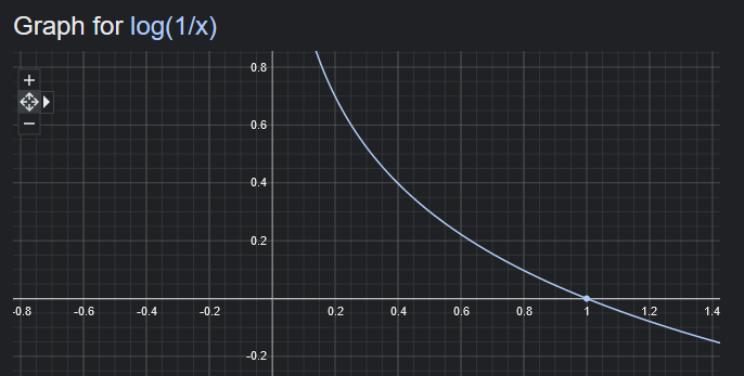
This is a much better expression, as now, when the probability is 1 for a certain event, the surprise is 0.
And if the probability for an event is closer to zero (unlikely to happen), then the surprise is closer to infinity!
Entropy is then just expected surprise of a random variable X.
To calculate expected surprise, we use the expression for EV. (Expected Values)
\[ E[\text{Surprise}] = \sum_i log \left( \frac{1}{p(x_i)} \right) * p(x_i) \]
Now we can simplify this expression and derive the entropy expression that Shannon described in his paper in 1948, "A mathematical theory of communication."
Note that surprise is synonymous with uncertainty.
\[ \begin{equation} \label{eq1} \begin{split} \text{Entropy} & = \sum_i log \left( \frac{1}{p(x_i)} \right) * p(x_i) \\ & = \sum_i p(x_i) * log \left( \frac{1}{p(x_i)} \right) \\ & = \sum_i p(x_i) * ( log(1) - log(p(x_i))) \\ & = \sum_i p(x_i) * log(1) - p(x_i)*log(p(x_i)) \\ & = \sum_i - p(x_i)*log(p(x_i)) \\ & = - \sum_i p(x_i)*log(p(x_i)) \\ \end{split} \end{equation} \]
Visualizing entropy via Python
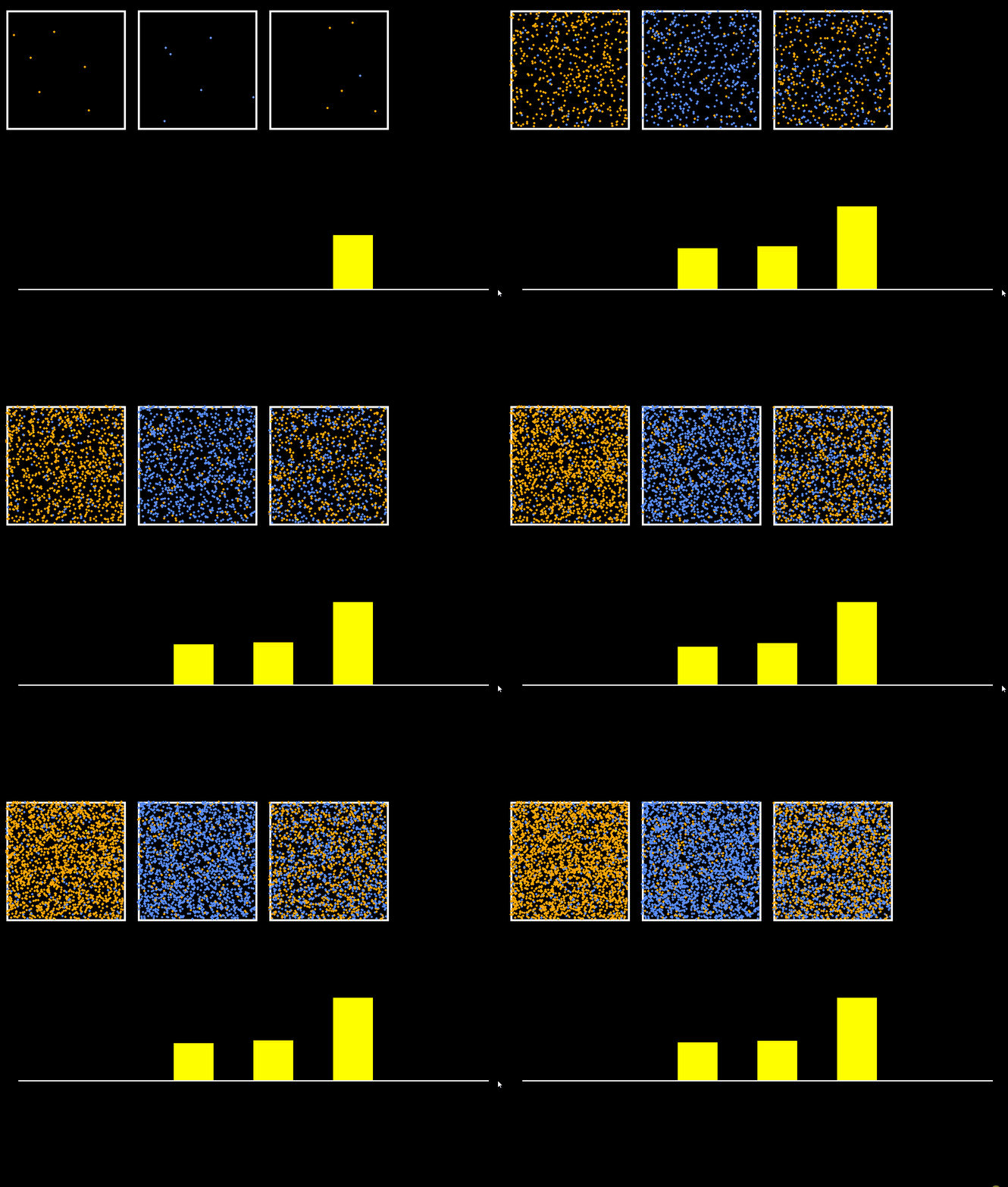
We have three boxes (pens) with orange and blue balls. Each box (or pen) has a different probability of how the balls spawn.
In the first box, more orange balls than blue balls would spawn.
In the second box, more blue balls than orange balls would spawn.
In the third box, both blue and orange boxes would spawn with a probability of 0.5. Both of them are equally likely to spawn.
The bars denote the amount of entropy for each box, respectively.
Since it's more likely that an orange or blue ball to spawn in the first and second boxes, their entropy is lower, as its uncertainty is less.
But in the third box, since we don't know the ball's color, that would spawn next, then the entropy is high, meaning the uncertainty is high.
The implementation code can be found in the following gist: https://gist.github.com/thenlpstudent/d20b5551568dcdbac9ba78d98e29ae24
Thanks for reading!
References
- A Mathematical Theory of Communication By C. E. SHANNON (shannon1948.dvi (harvard.edu))
- Stat Quest, Expected Values and Entropy
