The Multi-Armed Bandit Problem 

In solving the problem of exploration vs. exploitation in reinforcement learning, we use bandit problems to understand and apply algorithms that balance RL agents' exploration and exploitation behaviors. 

What exactly is the multi-armed bandit problem, and how can you solve this type of problem in RL? 

This blog post focuses on doing just that. 

What is the Multi Armed Bandit Problem? 

Consider the following situation that you find yourself in. 
You are faced repeatedly with 'k' different actions to take each time. 
After each action that you take at a given time, you receive a numerical reward.

This reward is picked out from a stationary probability distribution that depends on your selected action. 

Your goal in this problem is to maximize the total reward you receive over a period of time by selecting the best possible action at each time so that you maximize your reward. 

In this problem, each action has an average reward. This average reward is the value of the action, or how good that action is. 

If you knew the value of each action, then solving this problem would be very simple. Just pick the action with the highest value to get the biggest reward possible at the end. 

However, you don't know the value of each of these actions. Therefore, you would need to explore and come up with estimates on the value of each action by taking random actions in the first few timesteps. 

Once you have good guesses after the first few timesteps, then you are presented with a choice. 

Either you can exploit, which means pick the action with the largest value estimate or continue to explore and re-adjust your current estimates of the values of your actions. 

Stationary vs Non Stationary Bandit Problem 

The rewards for the actions you or the reinforcement learning (RL) agent takes at the current timestep are sampled from a probability distribution. E.g., Gaussian Distribution. 

In a stationary Bandit problem, the probability distribution doesn't change at each timestep, which means that the true value of each action is constant across all timesteps. However, in a non-stationary bandit problem, the probability distribution changes at every timestep. 

Therefore the true value of each action at each timestep is quite different from other timesteps. 

However, we can solve both variations of such bandit problems by estimating the value of each action, continuing to re-estimate them by trying different actions (exploration), or picking the highest calculated value action you currently have (exploitation) 

Solve by taking estimates 

One way to solve the Multi-Armed Bandit problem is through estimating the true value of each action.

Solving by estimating the true value of each action can either be applied to stationary and non-stationary bandit problems. 

Firstly we need a few mathematical notations to formalize the bandit problem before finding a way to solve it.

• \( A_t \)  The action the agent picks at time \(t\)
• \( R_t \)    The reward the agent earns at time \(t\)
• \( q_*(a) \)   The true value of action \(a\)
• \( Q_t(a) \)   The estimated value of action \(a\) at timestep \(t\) 

After exploration, we would want our RL agent to find closer estimates to the true value of action 'a'. 

\[ Q_t(a) \approx q_*(a) \]

To estimate the value of each action, we keep track of the total sum of rewards collected when we took a specific action 'a' and the number of times we took that action 'a'.

By dividing as follows, we get an average estimate of how good that action is at the current timestep. 

The below shows our definition for how the agent picks the suitable action at timestep t. 

This equation is the greedy approach (exploitation) in which the agent selects the highest estimated action value as its next action. 

The agent picks the action with the highest estimate, hoping that it would bring the highest possible reward for timestep 't'. 

Incremental Updates

To keep things simple let us assume the following change in notation, 
  

Since the above is computationally costly, we can incrementally compute the mean by re-arranging the mean calculation using a little bit of algebra. 

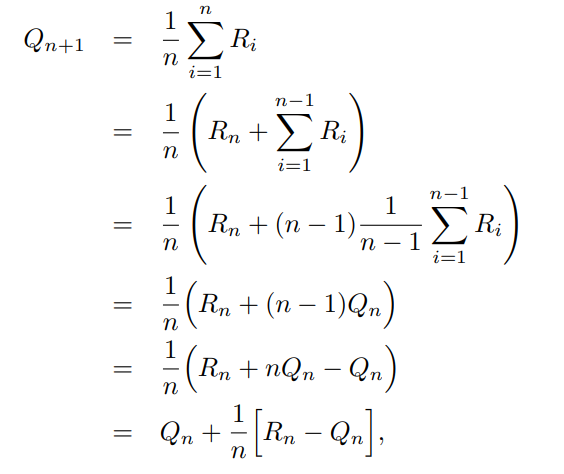
This mean update has the following form used throughout in reinforcement learning for problems other than bandits. 

The new estimate of the value of an action is the old estimate moved in the direction of the error between the current reward seen (i.e., 'target') and the old estimate. 

Solving non-stationary bandit problems 

When the optimal value changes from timestep to timestep, then you have a non-stationary bandit problem.

The probability distribution in which rewards are sampled from the agent for the action it picks comes from a different probability distribution randomly at every timestep.

Therefore the true value of each action is different at each timestep. 

Therefore we cannot rely on average sampling.

We need a mechanism in which we give more weight to rewards that we see recently instead of values we saw in the past and move the estimates of our action values towards recently seen reward signals. 

This is done using a fixed step size parameter \( \alpha \), a constant parameter that lies between 0 and 1. 

$$\begin{aligned} Q_{n+1} &= Q_n + \alpha[R_n + Q_n] \\ &= \alpha R_n + (1 - \alpha)Q_n \\ &= \alpha R_n + (1 - \alpha)Q_n \\ &= \alpha R_n + (1 - \alpha)[\alpha R_{n-1} + (1-\alpha)Q_{n-1}] \\ &= \alpha R_n + (1 - \alpha)[\alpha R_{n-1} + (1-\alpha)Q_{n-1}] \\ &= \alpha R_n + (1 - \alpha) \alpha R_{n-1} + (1 - \alpha)^2 \alpha R_{n-2} + .... + (1- \alpha)^nQ_1 \\ &= (1- \alpha)^nQ_1 + \sum^{n}_{i=1}\alpha(1 - \alpha)^{n-i}R_i \end{aligned}$$

By having a constant step size, the action values are updated so that the estimates are moved in the direction of the recent reward, as they have a higher weight and the older reward signals have a lower influence in the direction of where the estimates would move. 

This makes the RL agents get more good action value estimates in non-stationary bandit problems. 

Pseudocode, Code, and Results 

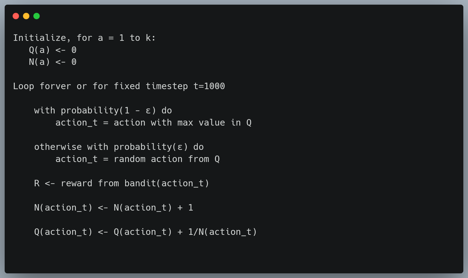
The following code snippet shows the pseudocode implementation of solving the bandit problem by estimating the value of each action. 

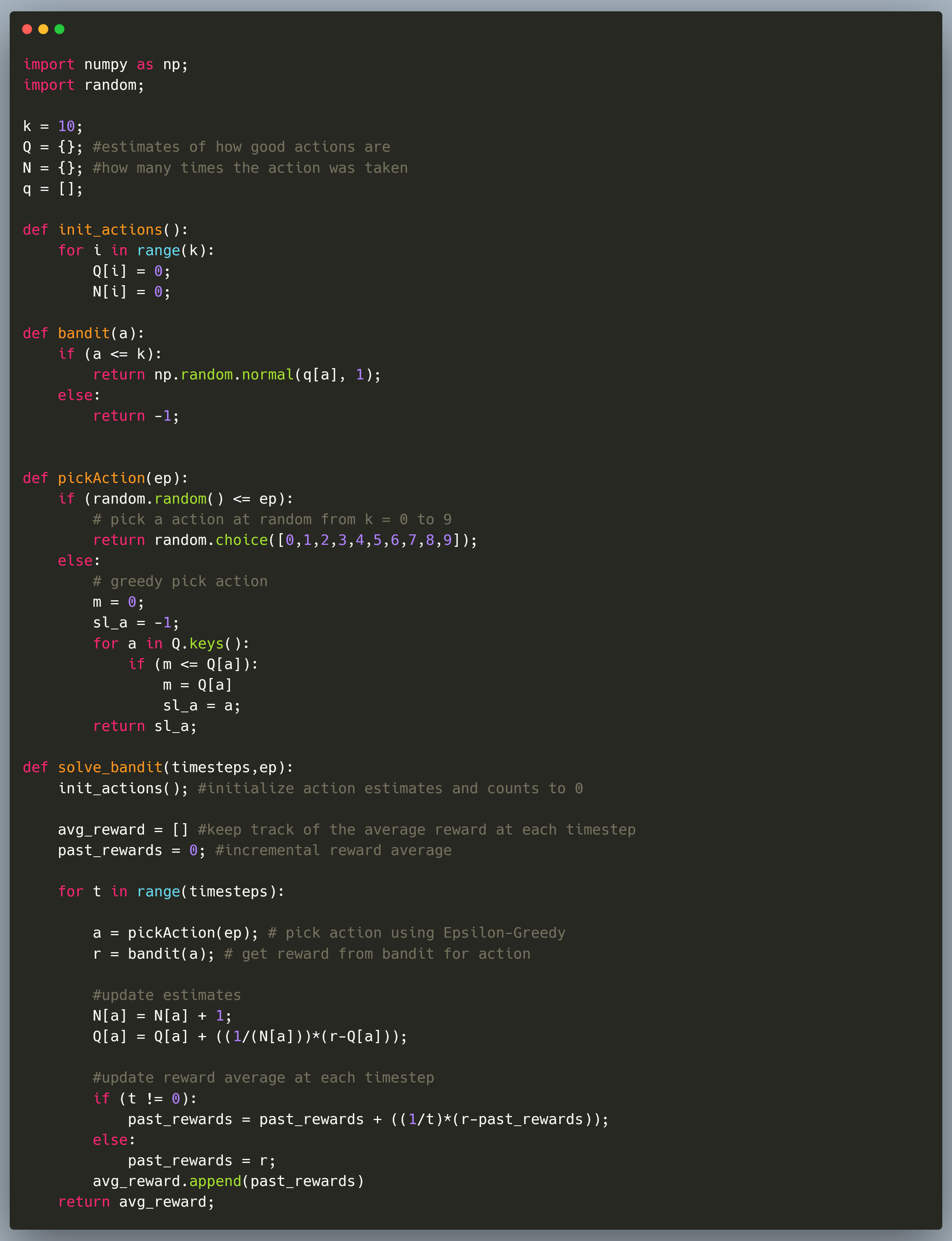
The following code snippet is the complete implementation of solving a ten-armed bandit problem. At each timestep, the agent can pick any ten actions and get a reward based on a gaussian distribution. 

This distribution doesn't change over timesteps. Therefore, this is a stationary bandit problem. 

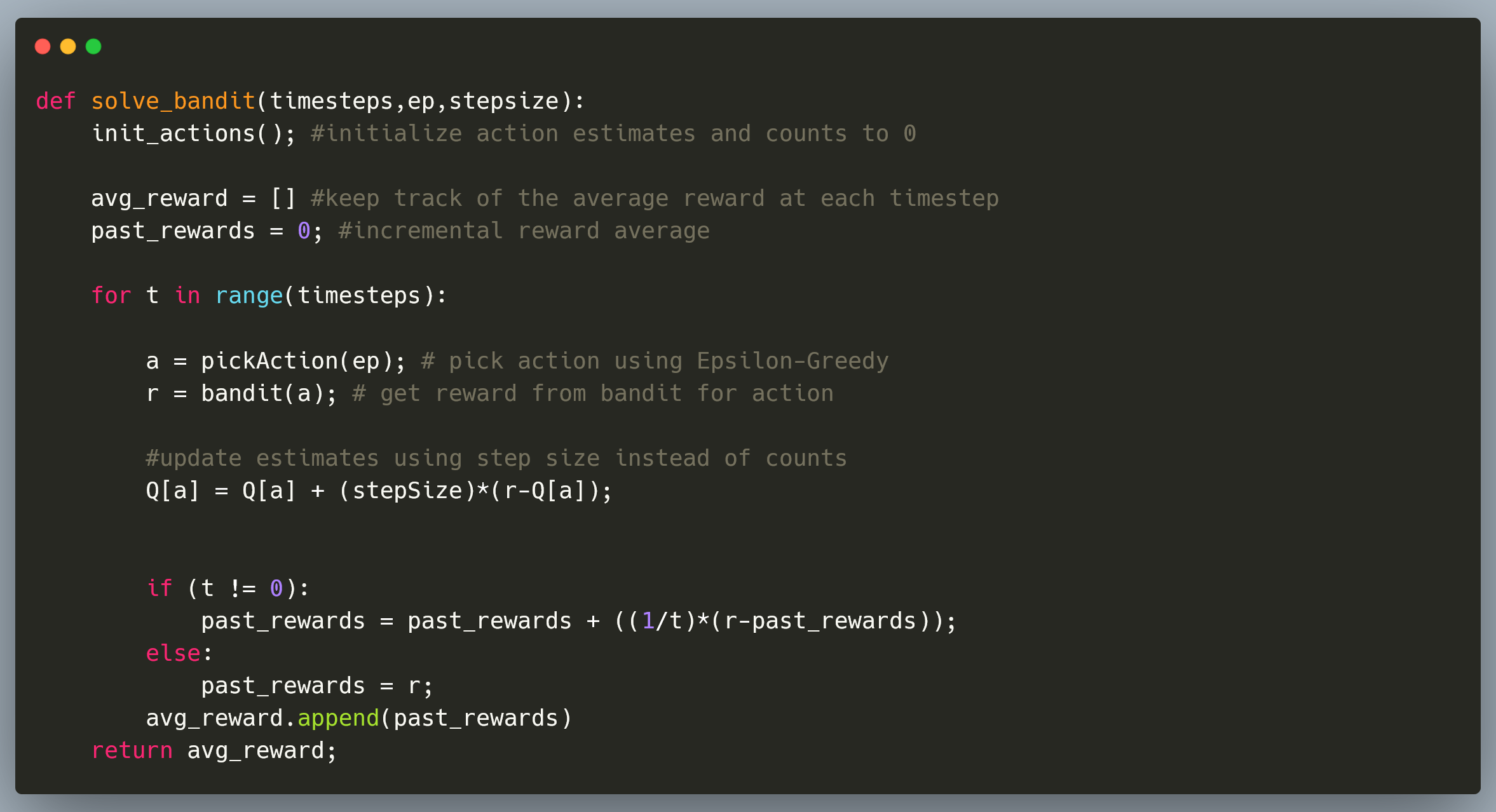
The following code snippet is modified slightly to show how we can solve a non-stationary bandit problem.

We can solve the problem using a step-size constant instead of counting how many times action 'a' was chosen before timestep t. 

The average reward at each timestep is stored in a list for each timestep.

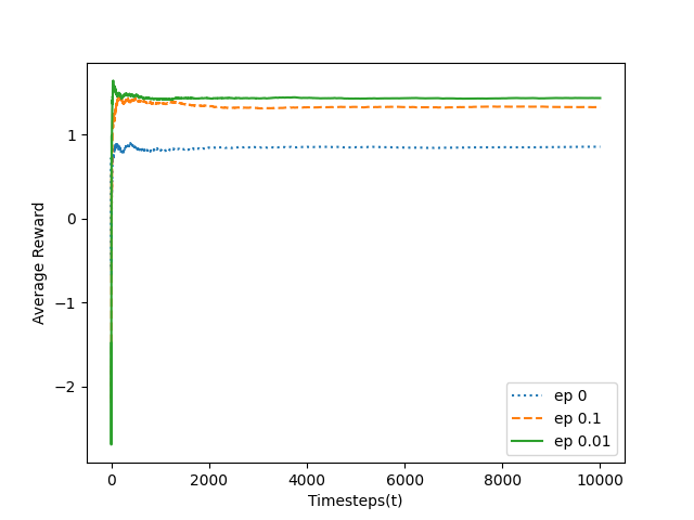
For example, the following graph shows how the epsilon parameter influences the epsilon-greedy algorithm to obtain high amounts of rewards over 10,000 timesteps. 

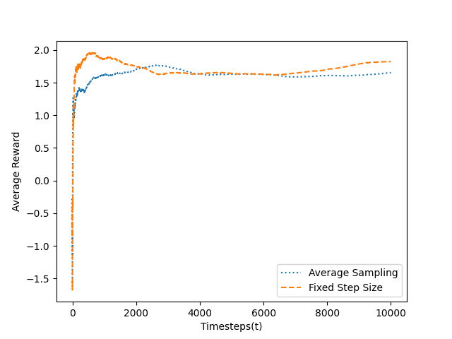
The graph below shows how average sampling methods with a variable step size perform compared to fixed step size sampling methods for non-stationary bandit problems. 

Thanks for reading this article this far! 

Follow me on Twitter @studentnlp so you won't miss my latest blog post, and as always, happy hacking!

References 

Sutton, R.S. & Barto, A.G., 2018. Reinforcement learning: An introduction, MIT press.