Basics of Reinforcement Learning: Part I
Welcome! In this article, we will be going over the fundamentals of reinforcement learning. We will discuss what reinforcement learning is, how agents learn from rewards and experiences, what policies and value functions are, and how to model environments in a Markov decision process step-by-step.
Table of Contents
What is Reinforcement Learning (RL)?
Reinforcement learning is a learning process in which agents learn through interacting with the environment and learn to take actions in a way that maximizes its reward signal. The reward signal is given by the environment depending on how well the agent performed in that environment.
Reinforcement learning is a computational approach that learns from interaction with an environment. The goal of a reinforcement learning agent is to maximize a numerical reward signal.
What is a reward?
A reward is a simple number given to the agent by the environment each time the agent interacts with the environment. The agent's goal is to maximize then the total amount of reward it receives, which means that the agent needs to maximize the cumulative reward in the long term, not the immediate reward in the short term.
The Reward Hypothesis
The reward hypothesis states that an RL agent's goal is to maximize the expected value of the received scalar signal's cumulative reward.
Therefore, reinforcement learning gets based on learning methods that maximize the total cumulative reward by taking actions that help reach this goal.
Components in Reinfocement learning
The two main components in any reinforcement learning-based algorithm are known as the agent and the environment.
The Agent and the Enviroment
An agent is a learner and the decision-maker inside an environment. The agent observes the environment and takes action, which is how the agent interacts with the environment. The environment then gives a reward to that agent based on the agent's action at that particular time and situation.
Everything that is outside of the agent is known as the environment.
What is the Markov State?
In RL, understanding the concept of a state is vital. The state is the information that we use to determine what might happen next. Simply put, the state is a function of history.
The agent has its state, in which case the agent's state is the function of the agent's history and experiences collected by interacting with the environment.
The environment also has its state, known as the environment state.
The agent's or the environment's state is a Markov state if the current state is independent of the past. This is because the past information (history) gets derived from the current state. Therefore the state doesn't depend on history.
"The future is independent of the past given the present" - and future states can be computed from the current state, and the history can be discarded.
Suppose the agent can access the environment state. In that case, the mathematical model of the RL problem is known as a fully observable Markov decision process, whereas if the agent cannot access the state of the environment, then it's known as a partially observable Markov decision process.
Returns, Epsoides and Continuous Tasks
The agent's goal is to maximize the total cumulative reward it receives from the environment over time.
To understand more about the return, we formalize it as follows. This is the basic form of the expected return, which is just the sum of all rewards gathered till the agent reaches the terminal state of the environment (last state of interaction with the environment) from some timestep t. Capital T denotes the final timestep.

Depending on the environment, the agent can work in episodic tasks or continuing tasks.
An episodic task ends at a specific terminal state S+ with different rewards for different outcomes. (All nonterminal states denoted as S.)
E.g., winning and losing a game of chess, the next episode or next game begins independently of how the previous game ended) The terminal state ends, and the environment resets back into a starting state.
Continous tasks don't have a terminal state. Therefore they go on without a limit. Here taking the total cumulative reward is tricky because the total cumulative reward will be T = ∞.
Now we introduce a notation known as the discount factor, a value between 0 and 1. This is so that in continuous environments, the total cumulative reward would not be ∞.
If we set the discount factor closer to 0, the agent tends to try and optimize to get higher immediate rewards. On the other hand, if the discount factor is closer to 1, the agent looks ahead to long-term rewards.
Therefore the agent now tries to select actions that maximize the sum of the discounted rewards (discounted return) it receives from timestep t onwards. So at each state, the agent tries to pick the best action at timestep t that maximizes the expected discounted return:

In the following manner, the current expected discounted return at timestep t relates with the future discounted return at time step t+1.
Thus, the current expected discounted return is the immediate reward at timestep t plus the discounted expected return at time step t+1.

What are value functions and policies?
Two other essential concepts in Reinforcement Learning are the value function and the policy function of an RL agent.
The value function of an RL agent describes how 'good' a state is in the long run.
It's a function that maps a state to a value that describes how much total expected discounted return the agent would get if the agent takes actions starting from that given state.
The policy is a function that maps a state with a given action.
Next, it describes how the behavior of the agent would be in the environment. Finally, it defines a way in which the agent would interact with the environment.
The policy function can either be discrete or stochastic, in the sense that it can map to certain actions based on an argmax function, where it picks the action that has the highest return (a greedy policy), or picks an action based on a probabilistic distribution.
The Markov Decision Process (MDP)
The Markov Decision Process is a classic formalization of sequential decision making, where actions influence the immediate reward at time step t and future states those actions and the rewards at those future states.
The MDP process formalizes and helps us derive equations on dealing with the trade-off between immediate and delayed rewards.
There are two types of values that we estimate by using an MDP, so that we can better deal with the immediate and delayed reward trade-off.
We estimate the optimal value function that gives each state S's best possible value given optimal action selections.
We also estimate the optimal action-value function, which takes in as arguments the action and the state the agent is in and gives how good of an action that action is depending on the state.
Estimating these state-dependent quantities is essential to accurately assign credit to the agent's actions in the environment to make decisions better to effectively trade-off between immediate and delayed rewards.
The agent would observe the current state at time step t and get the current reward from transitioning into that state. Then, the state would take action, which hopefully maximizes the discounted return for the next timestep.
The environment would process this action if the environment would produce the next state and reward the agent for moving into the new state.
This is how the agent and the environment interact with each other. The agent's goal is to behave optimally in this environment, which is done by maximizing the total discounted return over time.
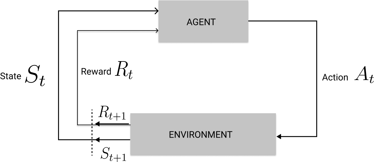
While interacting with the environment, this would be the sequential history the agent goes through.
For example, the agent starts at timestep 0, observes the state, takes action, and obtains a reward, and this cycle repeats.

The MDP describes the probability in which the agent transitions from one state to the next.
The likelihood that given the agent is in a given state 's' and takes action' a', the likelihood that that agent would end up in a new state " s' " and gets a reward 'r' is described as follows,


The expected reward for choosing action a from state s can be described as the summation of all rewards in R weighted over all the state transition probabilities from state 's', taking action 'a', landing in the state " s' " and getting a reward 'r' afterward.

The expected reward the agent will receive at the current state " s' " given that the previous state and action was 's' and 'a', is the summation of all rewards R, weighted by the total probability of transitioning from state 's' to " s' " by taking action 'a' over the probability of transitioning from state 's' to " s' " by taking action 'a' and getting a specific reward 'r' in R.

Here it shows that the probability of transitioning from all states " s' " and getting all rewards 'r' from those states given that the agent was in state 's' and takes action 'a' sums to 1. This shows that the function 'p' specifies a probability distribution for each choice of state 's' and action 'a'.

The Value Function
The value function defines how good it is to be in a particular state.
This means it gives the total expected discounted reward that is possible to receive, given that the agent continues to take actions from that state onward.
The value function depends upon the state, and the policy the agent follows since the selection of actions from state 's' onwards depends on the agent's policy or behavior.
The below equation shows that the value function when the agent uses a given policy π and starts at state s, is equivalent by the MDP to the expectation of the total discounted return from timestep t onwards, given that the agent currently at timestep t is on the state 's'.
Afterward, we can expand the definition of the total discounted return and show that this is true for all states in the MDP.

We can also evaluate this expectation as follows by the recursive defintion of the total discounted return.
Here it shows that the value function is the summation of all actions that can be made by the agent, and the probability the agent will choose that action is weighted by the sum the transitioning probabiltieis of all states and rewards from state 's' by taking action 'a' multiplied by the immediate reward of the given transitioning probabilities plus the discounted value of the value function under policy π for the next state " s' ".

The Action-Value Function
The action-value function maps a state and an action to show how much expected total discounted return the agent will receive from the environment if the agent starts at state 's' and takes action 'a' from that time until the environment terminates.

Solving the MDP
Solving the MDP entails that we find the optimal value function or the optimal action-value function, which can be derived from the optimal value function in the MDP and allowing the agent to pick the best action that gives the highest possible action-value for the state that the agent is currently at timestep t.
The optimal value and action-value function
The optimal value function is the maximum value that can be obtained from the state s given under the policy, which enables the agent to choose such actions from that state onwards which maximizes the expected total discounted return from that state onwards.

The optimal action-value function is the maximum action value obtained from state 's' by taking action 'a' under the policy that enables the agent to choose such actions from that state and action onwards, which maximizes the expected total discounted return from that state, action pair onwards.

The optimal action-value function can be written in terms of the optimal value function as the expectation of the immediate reward plus the discounted optimal value of the next state given that the current state is 's' and the action taken from that state is action 'a'.

The recurrence relation of the optimal value function is the value of the maximum action 'a' that can be taken which is a summation of all the states and rewards in the sets S and R of the MDP, weighted by the transition probability of moving to those states obtaining those rewards multiplied by the immediate reward plus the discounted optimal value of the next state the agent would move to.
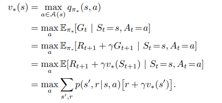
The recurrence relation of the optimal action-value function is the sum of all states and rewards in S and R of the MDP, weighted by the transition probability multiplied by the immediate reward 'r' plus the discounted best action-value function of the next state the agent would move into by taking action " a' " from that state.

Grid world Example
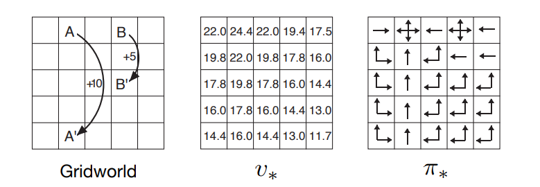
In this example, the RL agent has to traverse the following grid world, and any action that doesn't involve traversing from A to A' or B to B' gives a reward of -1. Otherwise, a reward of +10 and +5 is given if the agent gets teleported from A to A' or B to B'.
The agent can only take one step in north, east, south, and west.
While the agent updates its value function by interacting and moving in this grid world environment, the value function over time would update as shown in the below table.
It shows how much discounted total return each cell would give the agent over the long run.
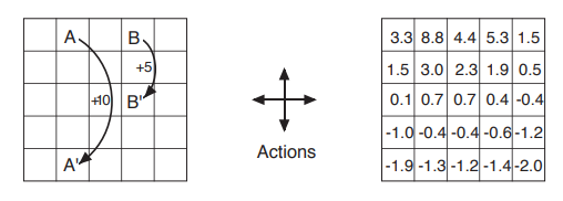
Once the agent finds the optimal policy that makes the agent optimize on getting the best possible discounted returns from this grid world, the value function would converge to the optimal value function.
By acting greedily upon the optimal value function, we find the optimal policy function.
If the agent chooses actions that get to better states (cells) with a higher value than the other states accessible from the current state the agent is in, the agent has successfully found the best policy to act optimally in this grid world in the below diagram.
That brings us to the end of the basics of reinforcement learning part 1.
This would be a 3 part series. In the second post, we will be going over Multi-armed bandits, an interesting problem in Reinforcement Learning. In the 3rd and final post, we will be going over finding the optimal value function solving the MDP using Dynamic Programming.
Stay tuned, and follow me on Twitter @studentnlp, so you don't miss any new posts.
Cheers!
References
- Sutton, R.S. & Barto, A.G., 2018. Reinforcement learning: An introduction, MIT press.
- David Silver "Introduction to Reinforcement Learning" DeepMind 2015
