The Transformer Explained

Welcome! In this article, we will be going over what a Transformer is, the intuition and the inner workings behind the attention mechanism it employs to process sequential data, and how the Multi-Head Attention mechanism works as implemented by the paper 'Attention is all you need' NeurIPS 2017. 

A transformer is a deep learning architecture that performs well for sequential data-related Machine learning tasks. It is based around an encoder-decoder architecture to handle and process sequential data in parallel. In addition, it uses a mechanism known as Attention to look back and forwards the sequential input and identify long-range patterns and relationships between each component in the sequence.

The transformer architecture solves the shortcomings of recurrent neural networks and convolutional neural networks when processing sequential data and making good predictions. 

Recurrent neural networks aren't capable of processing sequential data in parallel. Therefore it increases training time since we can't utilize the full power of GPU processing units for parallel matrix multiplication if data is processed sequentially.

Convolutional neural networks can also process sequential data in parallel. But due to their window size, they can only look back and forward the input sequence, making them unable to identify good long-distance relationships between the entire sequence. 

The attention mechanism can look at the whole input sequence at once and identify the long-distance relationships of every element (i.e. word) in the sequence with every other element of the sequence, which is why transformers, in general, perform better when it comes to sequential data processing. 

The Big Picture

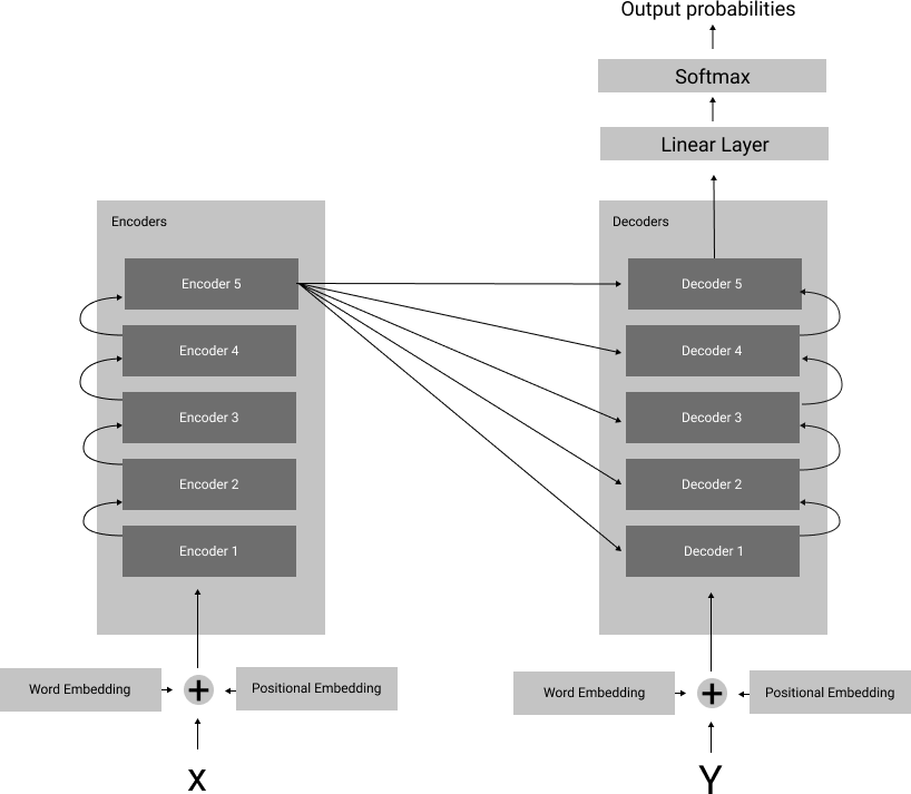
In a nutshell, the transformer uses an encoder-decoder architecture, where N (N=5 in the  different encoding layers encode the input sequences, and N different decoder layers decode the information encoded by the encoding layers to predict the next word in sequence, depending on the NLP task at hand.  

Before sending the input sequences into the encoder layers or to the decoder layers of the transformer, word embeddings and positional embeddings preprocess the input sequences so that the transformer can process the data more intuitively and effectively. 

 We will discuss the concept of word embedding and positional embedding once we dive more deeply into the inner workings of the transformer.

These encoder layers are stacked on top of each other. The last encoder layer creates an encoded embedding matrix that contains a representation of the learned sequence.

Finally, the decoder layer utilizes this matrix for a certain natural language processing task such as text classification, text generation, or machine translation. 

The original paper (Attention is all you need) utilized the transformer to convert English input sentences to German and French, proving that transformers are good at machine translation tasks. 

So let's dive deep into the inner workings of the transformers' encoder and decoder layers, how Attention works, and how supervised learning can train the transformer to optimize to perform better at machine translation and similar text processing tasks. 

How the Transformer works

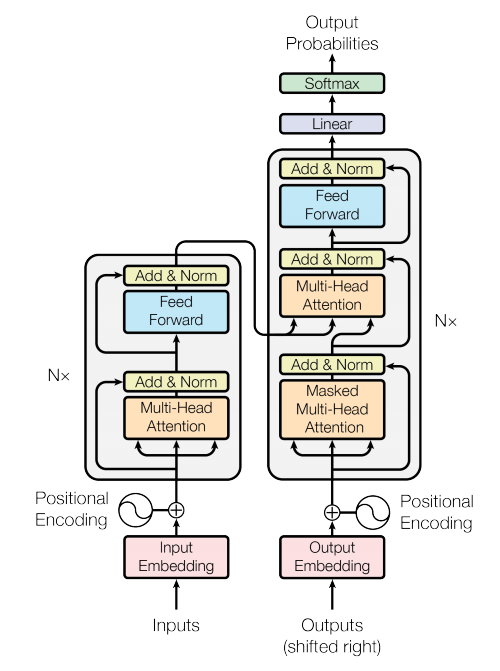
The paper that started it all by introducing the transformer at NIPS 2017 was called 'Attention is all you need', where Ashish Vaswani et al. proposed a deep learning model capable of processing sequences utilizing only Attention. Earlier variants of using Attention with sequence data involved connecting an attention layer to a recurrent neural network like a Long Short Term Memory (LSTM) network or a (Gated recurrent unit) GRU network. 

However, transformers proved that relying solely on the attention mechanism yielded better results, especially in the NLP problem area of language translation. 

Let's look at how the transformer processes information in a step by step manner and learns to make better predictions overtime. 

Step 1: Word and Positional Embedding 

The first step involves creating embeddings for the input sequences by word and positional embedding. 

Deep learning models can't process words the way humans do. They deal with vectors and matrices to make predictions. Therefore we must first convert words in the sequence into word vectors, representing a word in the vocabulary. 

Before the input sequences enter the encoders, the inputs are preprocessed and converted to word vectors, representing a word's contextual meaning in numeric form, so transformers can carry out numerical calculations to make predictions. 

When training a transformer, we have a set of vocabulary that we would like the transformer to learn. A vocabulary is a set of distinct words that you want the transformer to learn to do the NLP problem at hand effectively. 

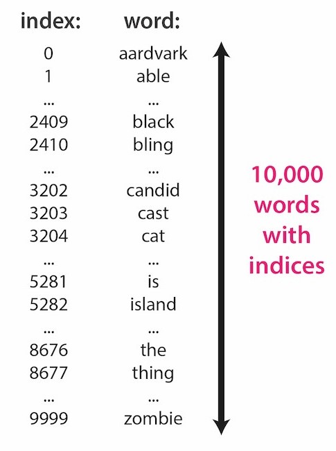
These word embeddings convert a given word to a word vector, which is a vector with a dimension of 'dᵐᵒᵈᵉˡ', which is a constant, or referred to as a hyperparameter of the network. The original paper had word vectors with the size of 512, which meant that to represent one word, the transformer converted each word into 512 numbers and stored them in vectors. 

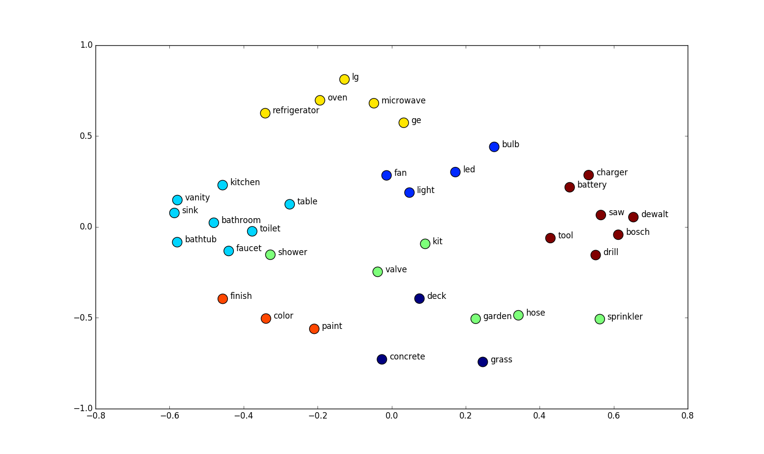
Word vectors can also be projected onto a 2-D plane, by shrinking their dimensionality from N dimensions to 2 dimensions. Once projected, the words that have similar context are grouped near each other.

Therefore to process the input sequence, we get the input word tokens from the sequence. We map each word to the location of the word in the vocabulary, assuming that the word is in the vocabulary. 

For example, the word index in the vocabulary could be 21; 21 is the word ID. So for every word in the sequence, we map it to its word ID. 

The below diagram shows multiple sentences with words being represented as a 2 dimensional matrix. 

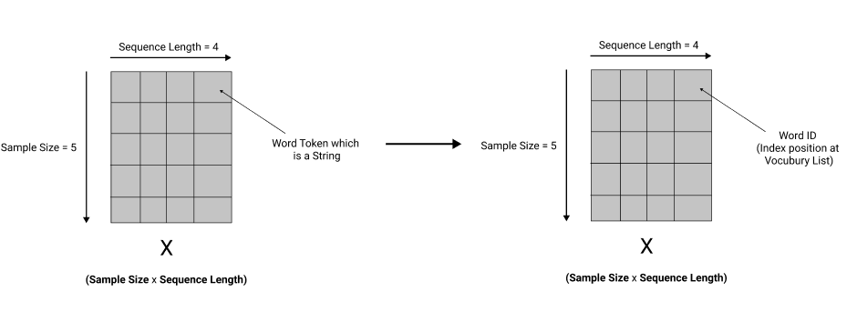
So our word tokens in the input sequences to the transformers are converted into word vectors, so the transformer knows the word's context when it processes it.

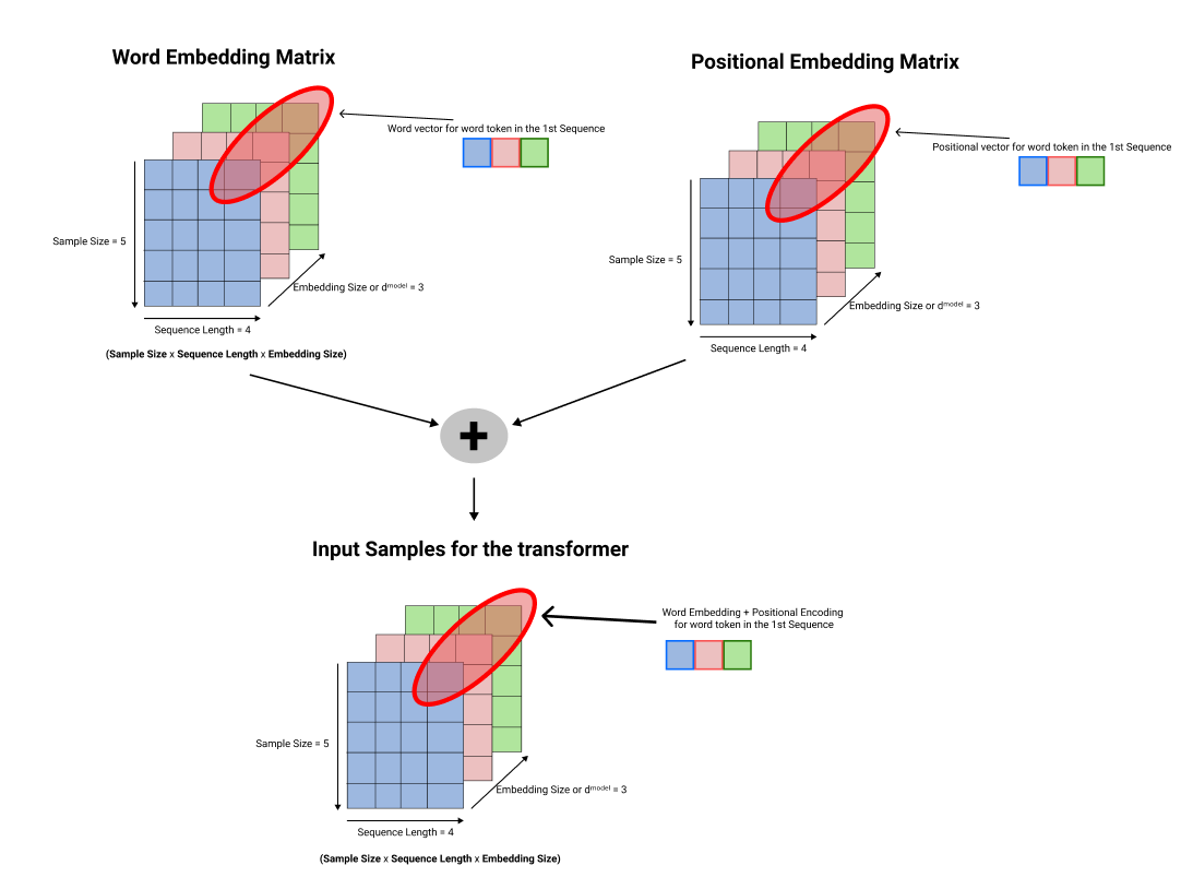
Once the word embeddings are created in this manner, positional encoding is also done to the input word tokens in the sequences before the sequences are sent off to the encoder layers.

Positional encoding tells the transformer what position the word vectors are in relative to each other in the sequence. Since sequences are processed in parallel, the transformer doesn't know beforehand what order the word vectors come in. In the perspective of a transformer, all words are in a similar position which is untrue. Therefore positional encoding encodes the word's relative position information into the representation before being processed by the encoder and decoder layers. 

Positional encoding is done using a sine and cosine function, and computed independtly of the word embeddings. 

• pos          : Position of the word in the sequence (or sentence) 
• d_model : Length of the word vector, also known as the embedding size 
• i              :  Index value of the word vector  

The sine function is applied to even indexes of i of the word vector, whereas the cosine function is applied to all odd indexes of the word vector. 

This diagram shows the big picture of word and position embedding done in the transformer

Step 2: Encoding Sequences using Attention

The N encoder layers encode the word vector sequences. Depending on the implementation the number of encoder/decoder layers can vary, the proposed transformer architecture in the paper has N = 6 encoder and decoder layers, stacked on top of one another. 

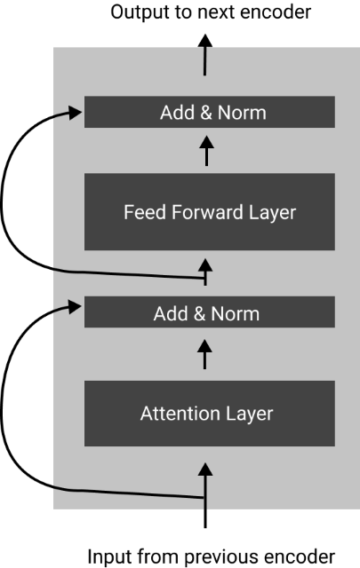
1. The input to the layer gets processed by an attention layer. 
2. An operation known as the 'Add & Norm' is done afterward, then the output is passed down to a feed-forward network.
   
3. Another 'Add & Norm' operation is done to the output and sent onto the next encoder layer.
   
4. The next encoder layer carries out the same operations, and the output is passed onto the next encoder on top of that afterward. 
   
5. The decoder layers utilize the output of the last encoder layer to generate the final output. 
   

What is attention? 

Before moving forward, it is essential to understand intuitively what the attention layer does in the encoder layer.

The attention layer tries to create a matrix that gives a score on how much each word relates to every other word in that sequence.

The following visual depicts what the attention layer tries to do to the input sequences. 

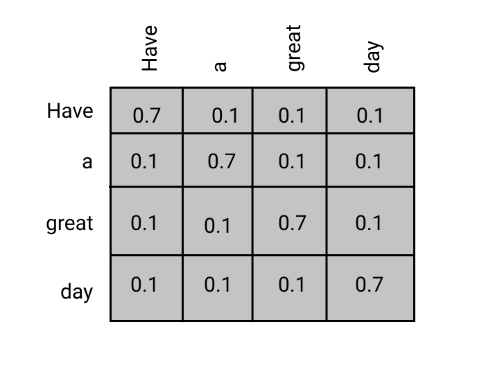
The following visual depicts what the attention layer tries to do to the input sequences. The attention layer lets the transformer model know where to focus on each word and its relation to other words. These long-range patterns are vital for various natural language processing tasks. Attention allows the transformer to look at the data at once and identify patterns effectively, which is why transformers perform better than RNNs.  

What is the 'add and norm' layer? 

The add and norm layer takes the output generated by the attention layer and the input for the attention layer, adds them together, and passes them as input to the Layer normalization function. 

"Layer Normalization directly estimates the normalization statistics from the summed inputs to the neurons within a hidden layer so the normalization does not introduce any new dependencies between training cases."

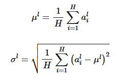
Here's the equation for the layer normalization function, where we first calculate the mean of the vector and using the mean, you calculate \row, which becomes the new input to the feed-forward layer. 

The feed-forward layer

The feed-forward layer in the encoder layer is a point-wise feed-forward network, a fully connected feed-forward network consisting of two linear transformations W1, B1, and W2, B2 with a ReLU activation function in between. 

The inputs for the feed-forward layer are d_model which is the embedding size, and the inner layer has a dimensionality of d_ff. The dimensions of the d_model and d_ff in the proposed architecture are 512, and 2048 respectively. 

Step 3: Decoding the input sequences 

The decoder layers are more or less similar to each other, but their behavior slightly changes when we use the model to train and when we use it for inference.

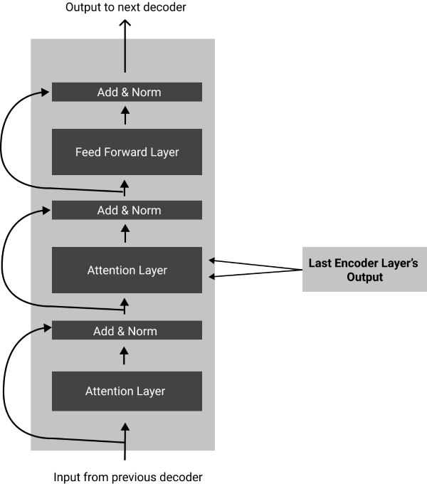
Like in the encoder layers, we embed the text input to the decoder layers, calculate their word vectors, and add positional encoding to it. We first input a 'START' token to the decoder layer to predict the next word in the sequence at the very end of the decoder layer.

The next word predicted by the decoder layers is ignored during training, only used for the loss calculation and backpropagation of the loss to optimize the weights of the transformer.

However, during inference, we append the predicted word as the next word token to our decoder layer and append it to the sequence to predict the next word at time step t+1. 

Each decoder layer has two attention layers; one is responsible for finding the connections of the output sequence's words with words that come before it, not after it. 

Then we send the output scores through an 'add & norm' layer, implemented in the same manner as the encoder layers. 

The next attention layer finds how relevant the words are in the output sequence compared with the input sequence from the encoder layer output.

The information from the second attention layer passes along onto another 'add and norm' layer, afterward a point-wise feed-forward layer, and finally through another 'add and norm' layer, and onto the next decoder layer above it. 

Step 4: Training and Inference 

The final decoder layer has a linear layer, a single linear operation applied onto the output of the last decoder layer, and maps the output of the decoder layer into a vector with the dimensions of the vocabulary size. (E.g. 10000)

A SoftMax function converts the values of that output vector into a probability distribution, and the index with the highest probability is chosen as the network's final output.

This chosen index position is mapped into the corresponding word by looking up the index from the vocabulary. 

In the training phase of the network, we calculate the next word and calculate the loss of the probability distribution of the SoftMax function with the target distribution. This loss is backpropagated across the network, and the weights of every decoder and encoder block are updated.

In the training phase, we use a method known as 'teacher forcing' where we manually input and append the correct word to the decoder layer's input sequence at each timestep to predict the next word.

During inference, the predicted next word is appended to the current input sequence of the decoder, and until a 'END' token is generated, the next word is predicted and appended to the sequence.

Understanding Attention 

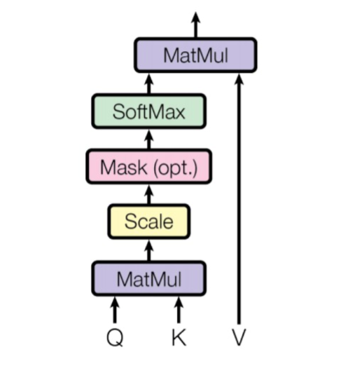
Attention is what makes the transformer understand long-range patterns in the sequence data that it processes and can make predictions considering the context of the input sequence and the relationships between each word vector in each sequence.

The self-attention mechanism compares every word token in a given sequence with every other word token in the sequence and gauges how much they are important to each other. 

They model the relationship each word token has with each other in the sequence. Whether that relationship is strong or weak, based on these attention scores, the feedforward layers of the encoder/decoder layer can make better predictions by understanding the dependency of each word token with the rest of the word tokens. 

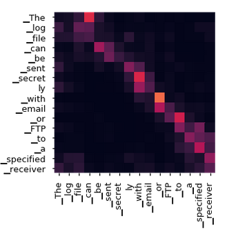
The below matrices shows how the attention layer scores word vector pairs based on how strong the relationships is between the two word vectors in the sequence. 

Note that each word's contextual meaning as well as positional information is taken into account when the attention layer computes the scores. 

The attention model works by comparing every word token with every other word token using the dot-product operation. The more significant the magnitude of the dot-product, the higher likelihood that the pair of word vectors have a strong relationship and vice versa. Thus, the attention mechanism functions as a lookup dictionary.

A dictionary has queries, keys, and values.
We match up the queries with the keys and weigh them. The higher the dot product of the query and key pair, the higher the likelihood of them relating to one another.

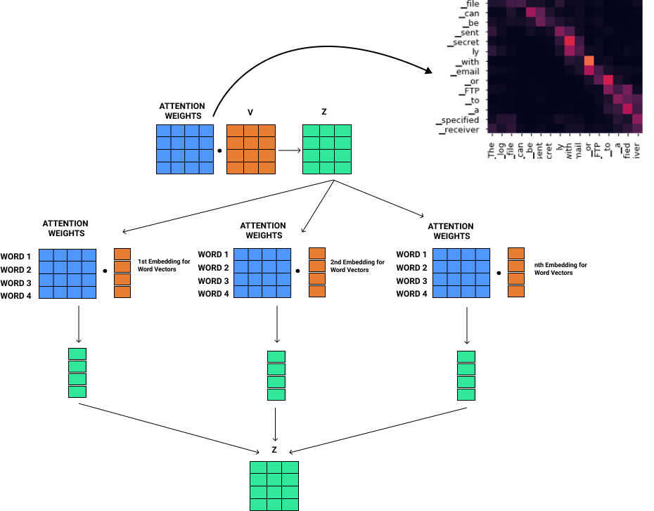
With the multiplication of the query and key pairs together with every Value vector in the Value Matrix, we find which word is most likely has a strong connection with which word in the sequence. 

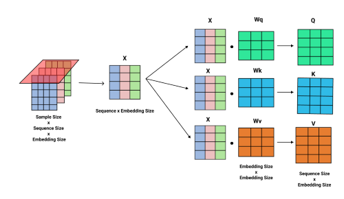
These query, key, and value are matrices created by multiplying the input sequence by weight matrices Wq, Wk, and Wv. These parameters are fine-tuned when the transformer trains, and over time the attention mechanism can learn the interrelationships between each word token for effective prediction over time. 

Here are the formulas that generate matrices Q for Query, K for Key, and V for Value. 

The below diagram shows how the matrix multiplication occurs visually 

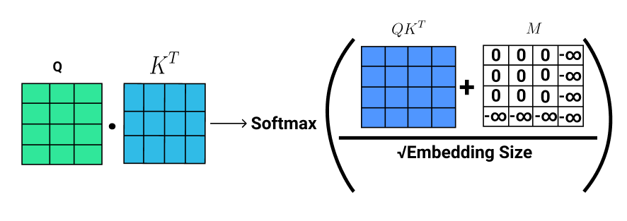
Here are the formulae that calculate the attention score for a given input sequence, where M is the mask matrix, which is explained in the next section. 

Masking 

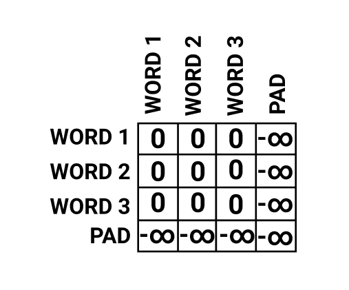
A design feature of attention is masking. When calculating attention, it's important that we only consider the attention scores of valid word vectors.

Some sentences might not be of the length as the sequence size in the encoder layer, and sentences can have varying lengths. So we add a unique token known as the 'PAD' token to make all sentences the same length. 

However, the 'PAD' token is meaningless. Therefore we don't calculate the attention score of that token. 

To cancel out the attention score of 'PAD' tokens, before we calculate the attention score using the SoftMax function, we add a mask matrix to the attention score.

A mask matrix in the encoder layer might look something like this.  

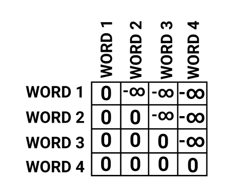
In the decoder layers, we want to force the network to only make predictions by looking at the word before it. Thus, we force the network to guess the next word in the sequence by looking back at the words before it. This type of mask is known as a look-ahead mask. 

Here's what a mask in the decoder layer might look like this.

Here's the complete visualization on how attention is calculated

Attention in the decoder layers 

In the decoder layer, we have an attention layer that relies on the encoder's input representation. 

The encoder's input representation takes the Query and Key values, and the value matrix is taken from the decoder's input. Intuitively this means that we find the relationship between the encoder's input word vectors and how it relates to the decoder's word vectors. 

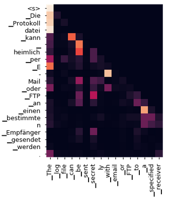
For example, in the context of machine translation, if you have English words as input and translating them into German, the encoder's input representation would be English word vectors, and the decoder's input representation would be German word vectors. We find the relationship between the encoder's input representation and the decoder's input representation, essentially finding out how strong or weak the relationship is between English and German word pairs. 

The below matrix shows how the attention layer gauges and compares every German word in the output sequence with every English word in the input sequence, and models the relationship between both the languages. 

Multi-Head Attention: cause n>1 heads are better than one! 

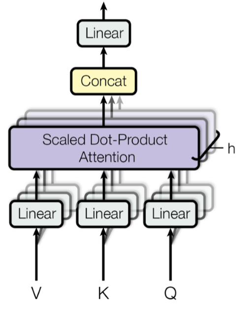
Multi-head attention splits the input sequence into multiple parts and applies scaled dot product attention to each part individually. 

This has been shown to improve the quality of attention as more complex relationships between word tokens can be extracted. 

The input sequence is split based on the number of heads, a hyperparameter set before training the transformer. 

For example, if the head size is 8, the input sequence is split into eight equal parts by dividing the embedding size by the number of attention heads. This is known as the query size.

Query size is equal to the embedding size divided by the number of attention heads. 

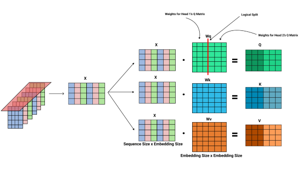
A linear layer is used to get the Q, K, and V matrices by multiplying the input matrix by the corresponding weight matrix. In this example, the embedding size is 6, and the number of attention heads used is 2. Therefore the query size is 6/2, which is 3. 

As you can see in the above diagram, there is a red line separating the weights of the two heads, which is known as the logical split. When implementing, each attention head doesn't have its weight matrix, but the weights for every attention head are in one matrix. Thus, it's designed to easily update the weight matrices without taking up much memory, compute power, or time. 

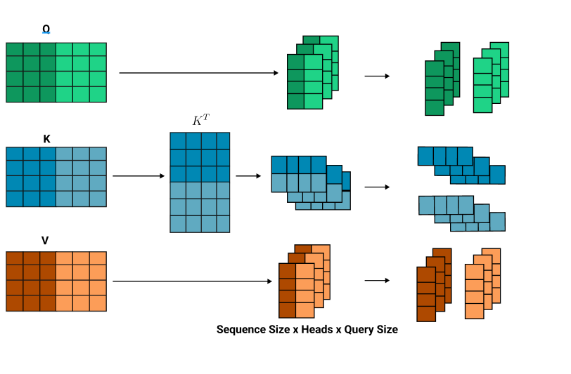
Same as before, the K matrix transposes to multiply the Q and K matrices together. 

However, before multiplying both these matrices, we first add an extra dimension known as the head size, which is 2 in this case. 

This turns the 2D Q and K matrices to 3 dimensional. The V matrix is also reshaped to have a head dimension. Therefore all matrices are reshaped to the form Sequence Size x Head Size x Query Size. 

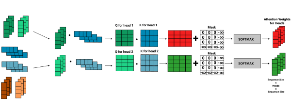
Afterward, we carry out the matrix multiplication for Q and K, where we multiply the matrices for each head, Q_head1 with K_head1 and Q_head2 with K_head2. 

Afterward, every matrix multiplication of Q and K for each head results in a matrix with the shape sequence size x sequence size. 

Finally, we add masks for each head's Q and K product, and we scale it by the square root of the query size and then apply a SoftMax function over it, creating separate attention weight matrices for each head, as show below.

Finally, we multiply the corresponding V matrix's heads with attention weight heads giving us attention scores for each head, as show below. 

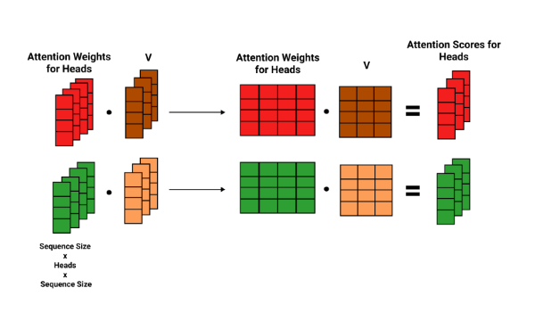
We need to reshape it back into its original form and merge all the results from the different heads into one by dropping the head dimension altogether.

First, we reshape the matrix into the form Sequence Size x Query Size x Head Size by swapping the head size with the query size, which alters the shape of the matrix to the following form.

We can get rid of the head dimension, which makes the 3-dimensional matrix back into two dimensions.

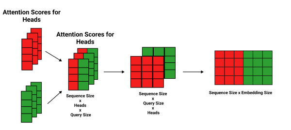
Afterward, we multiply the resulting merged matrix using a weight matrix W0 with a shape of embedding size x embedding size, and we add a bias vector to the resulting matrix.

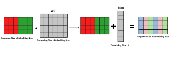
This is how multi-head attention is done to a single sample of our input. Likewise, we carry out the following process simultaneously for all sentence samples, thanks to the fact that matrix multiplication is inherently parallelizable. 

References 

• Attention is all you need - Ashish Vaswani et al, NIPS 2017
  
• Tensor flow model for language understanding